Sequential palettes

library(circadia)
library(ggplot2)
library(patchwork)

Sequential palettes map a continuous range from low (light) to high (saturated). circadia provides two families:

Family	Palettes	Hue strategy
Complex	blues, warm	Multi-hue — higher perceptual contrast
Simple	seq_blue, seq_coral, seq_amber, seq_ochre	Monochromatic shades — consistent hue identity

Use complex palettes when maximum contrast across the range matters. Use simple palettes when you want the colour to stay clearly associated with a particular brand colour throughout its range.

Complex sequential

blues

Six stops from deep blue to pale teal — suited to density, intensity, or frequency data.

#014370

#1B6799

#4A9BBF

#7FB5C8

#9BDFE2

#D4F3F5

ggplot(faithfuld, aes(waiting, eruptions, fill = density)) +
  geom_tile() +
  scale_fill_circadia_c("blues") +
  labs(title = "Old Faithful eruption density — blues",
       x = "Waiting time (min)", y = "Eruption duration (min)") +
  theme_circadia(grid = "none")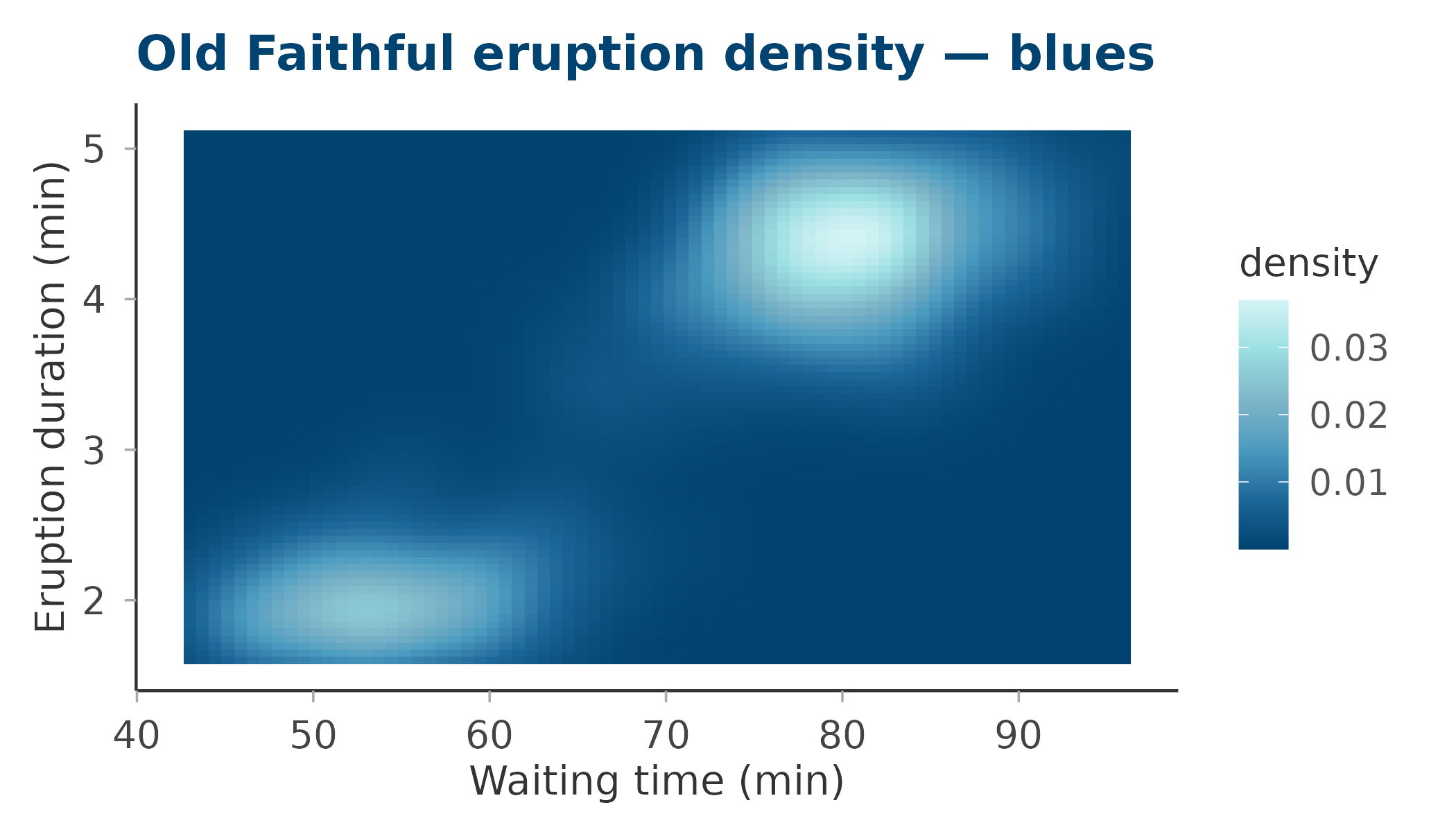

warm

Five stops from coral to antique white — suited to warm-toned data such as body temperature, light exposure, or alertness ratings.

#FC544A

#FC7060

#FFA75D

#FFC99A

#FFECD4

ggplot(faithfuld, aes(waiting, eruptions, fill = density)) +
  geom_tile() +
  scale_fill_circadia_c("warm") +
  labs(title = "Old Faithful eruption density — warm",
       x = "Waiting time (min)", y = "Eruption duration (min)") +
  theme_circadia(grid = "none")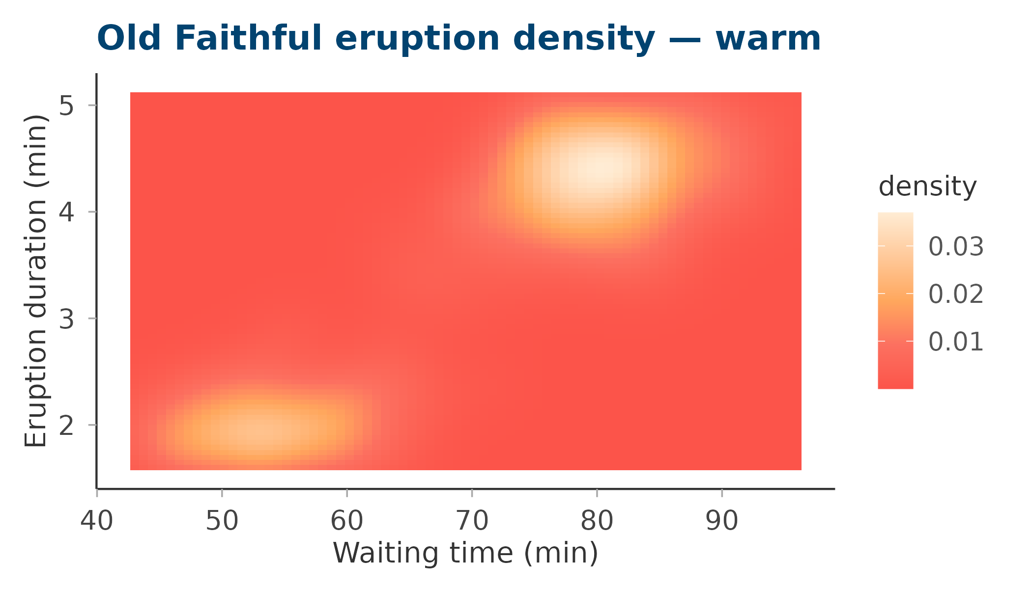

Simple sequential

Each simple palette is a monochromatic ramp of one brand colour, running from a pale tint to the full saturated value. Use these when the hue itself carries meaning — e.g. seq_blue for sleep depth, seq_ochre for light exposure intensity.

seq_blue

#D4E5EF

#8FBDD5

#4A95BB

#1B6799

#014370

seq_coral

#FDECE8

#F9B5AD

#F57E73

#F54840

#C22420

seq_amber

#FFF0E2

#FFC87A

#FFA016

#D97A00

#A85E00

seq_ochre

#F5E8C0

#E0BB6A

#C8860A

#9A6508

#6C4606

make_tile <- function(pal) {
  ggplot(faithfuld, aes(waiting, eruptions, fill = density)) +
    geom_tile() +
    scale_fill_circadia_c(pal) +
    labs(title = pal, x = NULL, y = NULL) +
    theme_circadia(grid = "none") +
    theme(
      plot.title = element_text(size = 11),
      axis.text  = element_blank(),
      axis.ticks = element_blank(),
      legend.position = "none"
    )
}

(make_tile("seq_blue") + make_tile("seq_coral")) /
(make_tile("seq_amber") + make_tile("seq_ochre"))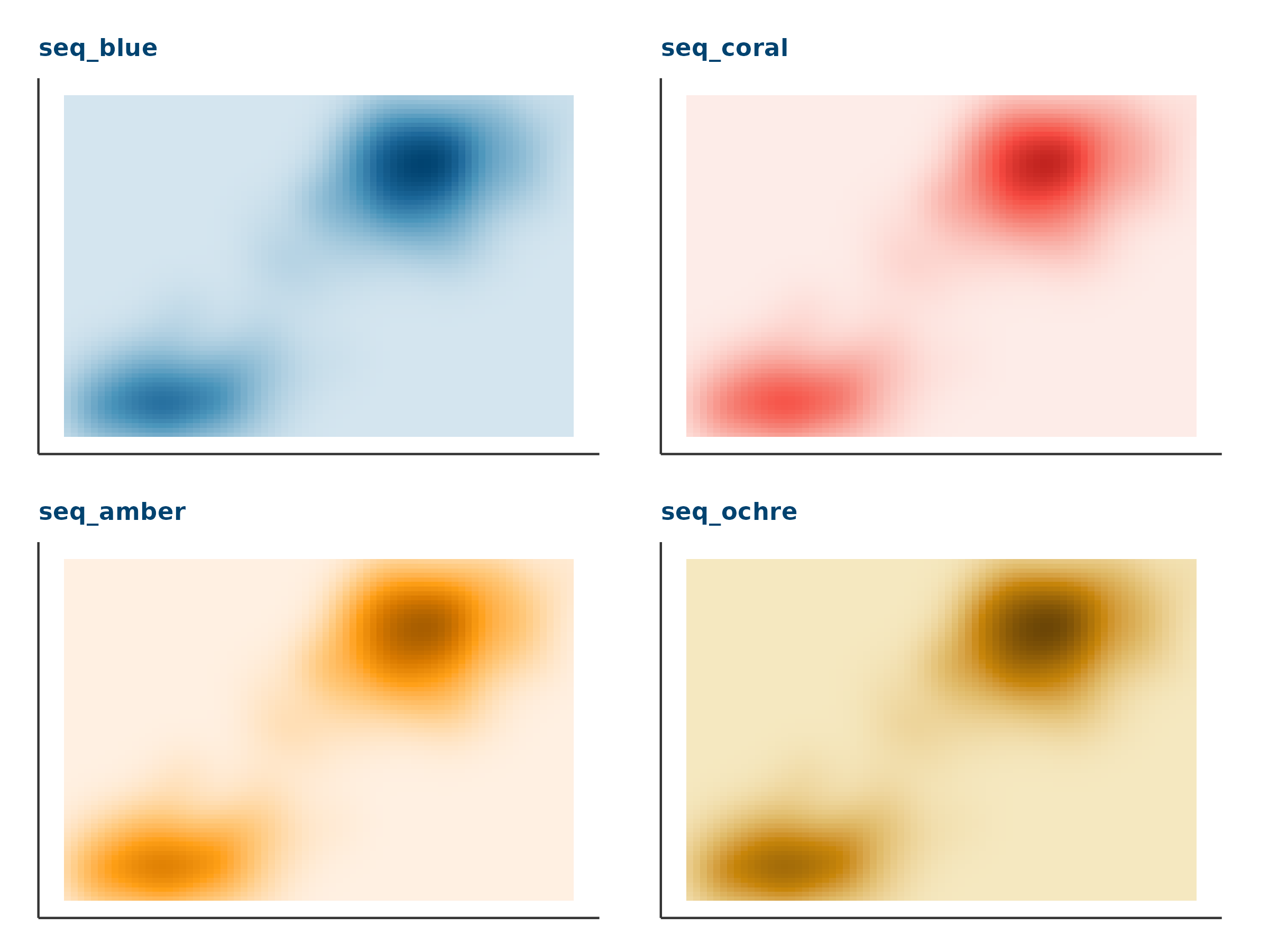

Combining with theme_circadia()

All continuous scales compose naturally with theme_circadia():

ggplot(mtcars, aes(wt, mpg, colour = hp)) +
  geom_point(size = 3) +
  scale_colour_circadia_c("blues") +
  labs(
    title  = "Weight, efficiency and horsepower",
    colour = "HP",
    x      = "Weight (1000 lbs)", y = "Miles per gallon"
  ) +
  theme_circadia()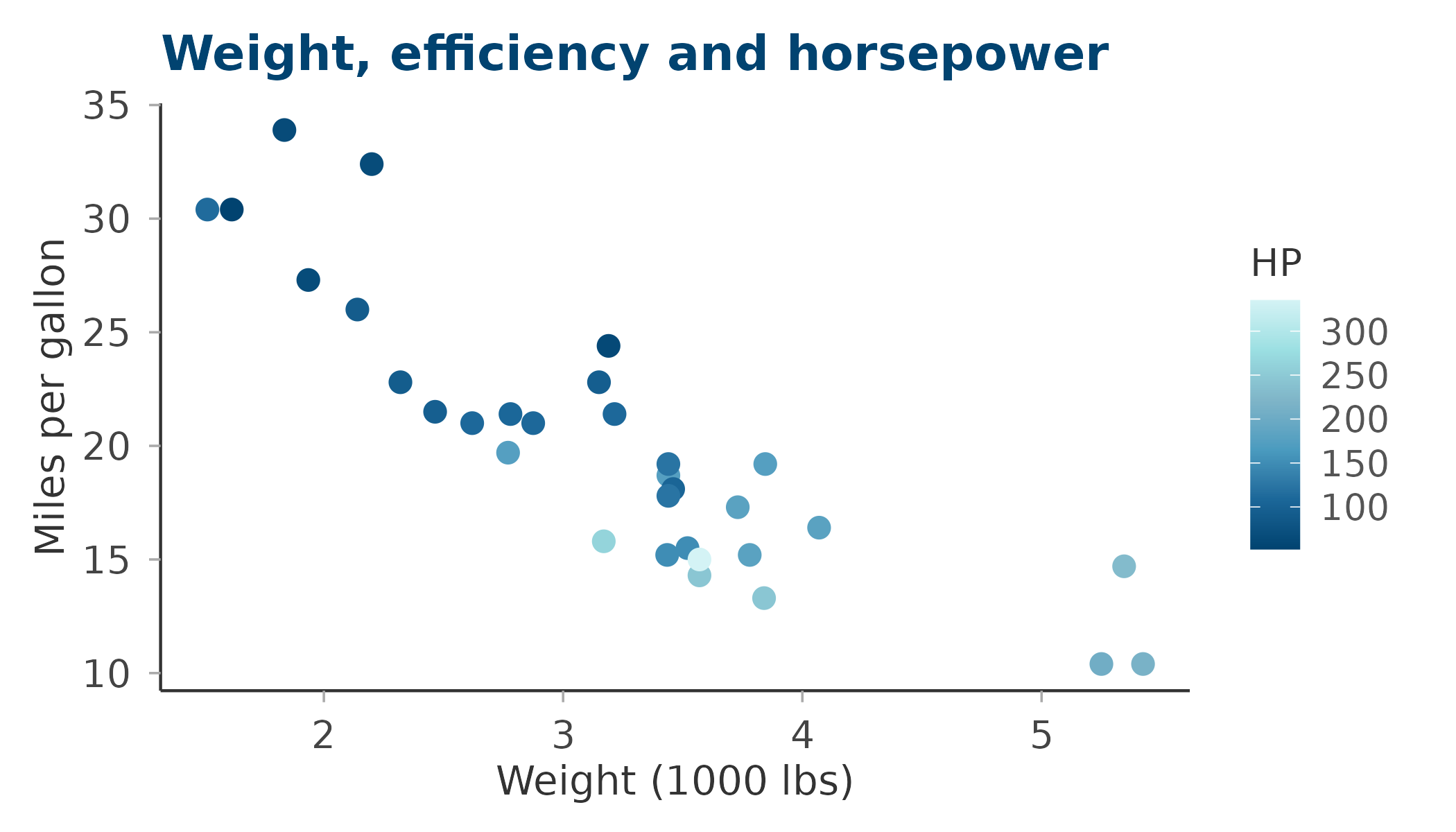

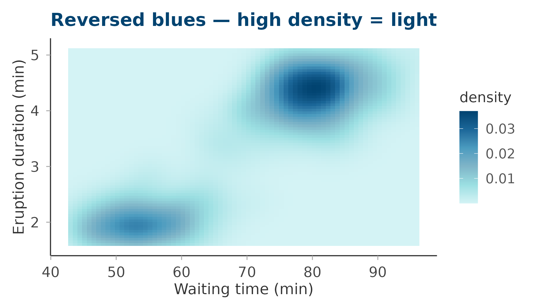
Reversing

Pass reverse = TRUE to any continuous scale to flip the direction — useful when lower values should map to the saturated end:

ggplot(faithfuld, aes(waiting, eruptions, fill = density)) +
  geom_tile() +
  scale_fill_circadia_c("blues", reverse = TRUE) +
  labs(title = "Reversed blues — high density = light",
       x = "Waiting time (min)", y = "Eruption duration (min)") +
  theme_circadia(grid = "none")