Getting started with circadia

The circadia package provides the shared visual identity for the Circadia Lab R ecosystem. It ships five colour palettes, a ggplot2 theme, and discrete/continuous scale functions that can be dropped into any plot across zeitR, slumbR, tallieR, or syncR.

library(circadia)
library(ggplot2)

Palettes

Retrieve any palette by name with circadia_palette():

circadia_palettes()   # list all available palettes
#> Available circadia palettes:
#>   Qualitative:
#>     main                  8 colours
#>     core                  5 colours
#>   Diverging:
#>     diverging             9 colours
#>     diverging_simple      7 colours
#>   Sequential (complex):
#>     blues                 6 colours
#>     warm                  5 colours
#>   Sequential (simple):
#>     seq_blue              5 colours
#>     seq_coral             5 colours
#>     seq_amber             5 colours
#>     seq_ochre             5 colours

circadia_palette()          # main (6 colours, default)
#>     deep_blue     coral_red         amber         ochre antique_white 
#>     "#014370"     "#FC544A"     "#FFA75D"     "#C8860A"     "#FFECD4" 
#>      mid_blue    steel_blue     pale_teal 
#>     "#1B6799"     "#4A9BBF"     "#9BDFE2"
circadia_palette("core")    # compact 4-colour subset
#>     deep_blue     coral_red         amber         ochre antique_white 
#>     "#014370"     "#FC544A"     "#FFA75D"     "#C8860A"     "#FFECD4"
circadia_palette("blues", n = 4)
#> [1] "#014370" "#1B6799" "#4A9BBF" "#7FB5C8"

All palettes support reverse = TRUE and sub-setting via n:

circadia_palette("diverging", reverse = TRUE)
#> [1] "#FC544A" "#FC7060" "#FFA75D" "#FFC99A" "#FFECD4" "#9BDFE2" "#4A9BBF"
#> [8] "#1B6799" "#014370"

Domain colours

domain_colour_for() maps data domains to their brand colour — useful when annotating panels by data type:

domain_colour_for("actigraphy")
#> actigraphy 
#>  "#014370"
domain_colour_for("sleep")
#>     sleep 
#> "#1B6799"
domain_colour_for("questionnaire")
#> questionnaire 
#>     "#FFA75D"

The theme_circadia() theme

Apply theme_circadia() to any ggplot2 plot:

ggplot(mtcars, aes(wt, mpg, colour = factor(cyl))) +
  geom_point(size = 3) +
  labs(
    title    = "Motor Trend Car Road Tests",
    subtitle = "Weight vs fuel efficiency by cylinder count",
    colour   = "Cylinders",
    x = "Weight (1000 lbs)", y = "Miles per gallon"
  ) +
  scale_colour_circadia() +
  theme_circadia()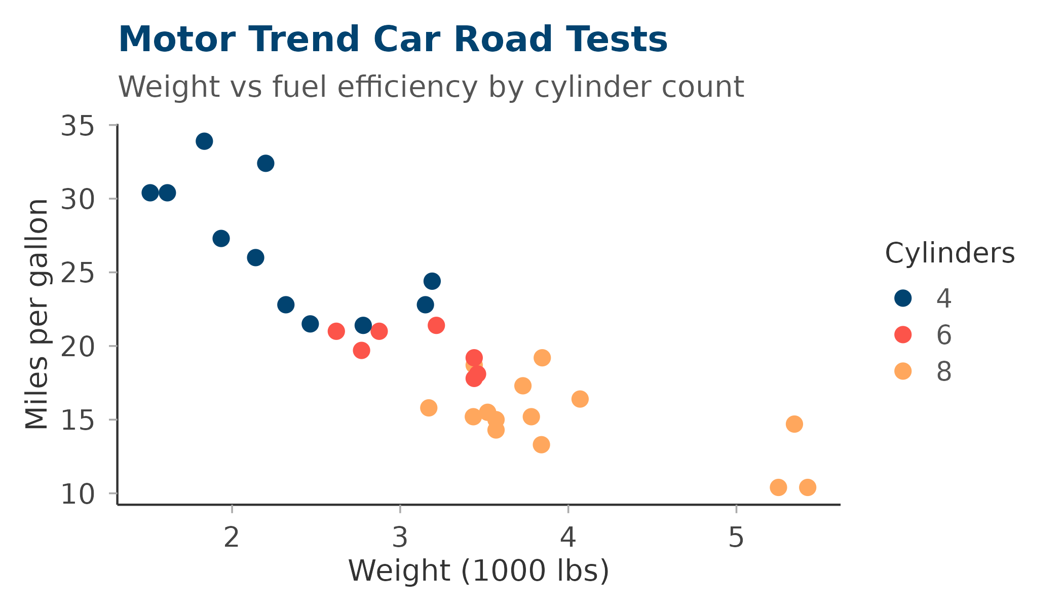

The grid argument controls which gridlines are shown:

ggplot(mpg, aes(class, fill = drv)) +
  geom_bar() +
  scale_fill_circadia() +
  theme_circadia(grid = "y", legend_position = "top")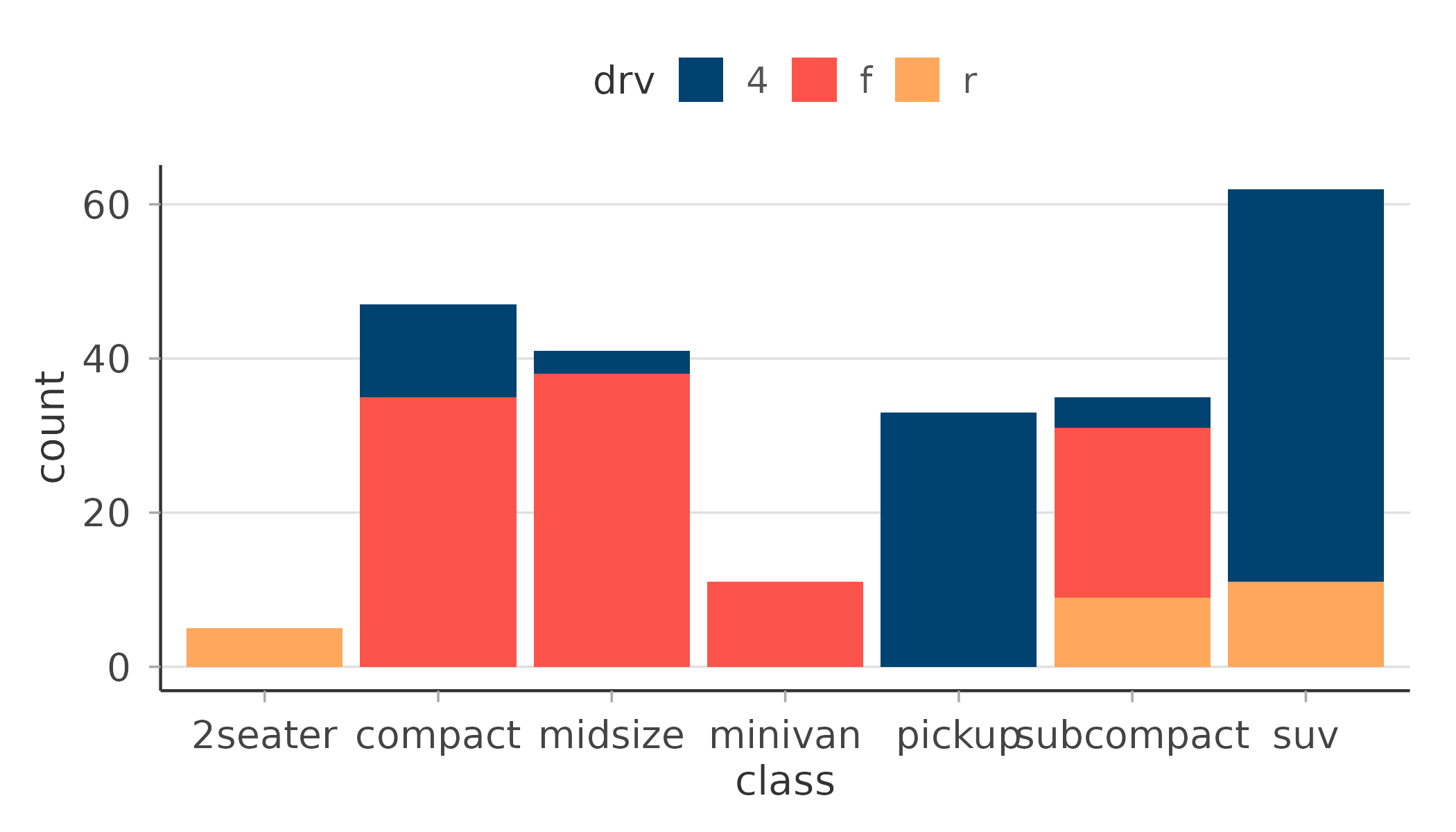

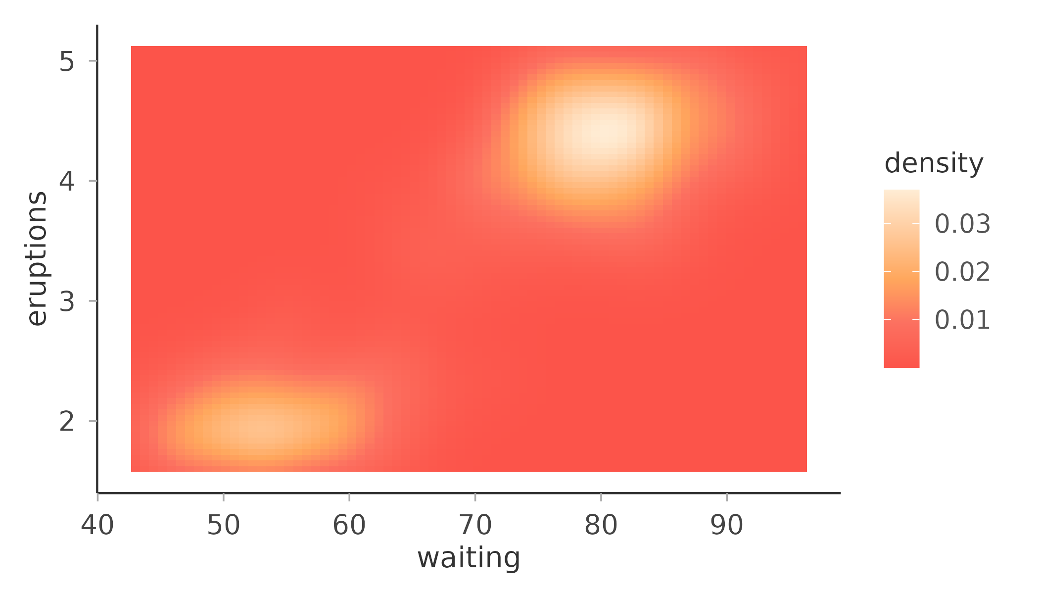
Continuous scales

For continuous data use scale_fill_circadia_c() or scale_colour_circadia_c(). The "diverging" palette suits centred data; "blues" or "warm" suit unipolar data.

ggplot(faithfuld, aes(waiting, eruptions, fill = density)) +
  geom_tile() +
  scale_fill_circadia_c("warm") +
  theme_circadia(grid = "none")